Diagonal Gauss-Newton Second order optimizer

A simple second-order optimizer with BackPACK on the classic MNIST example from PyTorch. The optimizer we implement uses uses the diagonal of the GGN/Fisher matrix as a preconditioner, with a constant damping parameter;

\[x_{t+1} = x_t - \gamma (G(x_t) + \lambda I)^{-1} g(x_t),\]

where

\[\begin{split}\begin{array}{ll} x_t: & \text{parameters of the model} \\ g(x_t): & \text{gradient} \\ G(x_t): & \text{diagonal of the Gauss-Newton/Fisher matrix at `x_t`} \\ \lambda: & \text{damping parameter} \\ \gamma: & \text{step-size} \\ \end{array}\end{split}\]

Let’s get the imports, configuration and some helper functions out of the way first.

import matplotlib.pyplot as plt
import torch

from backpack import backpack, extend
from backpack.extensions import DiagGGNMC
from backpack.utils.examples import get_mnist_dataloader

BATCH_SIZE = 128
STEP_SIZE = 0.05
DAMPING = 1.0
MAX_ITER = 200
PRINT_EVERY = 50
DEVICE = torch.device("cuda:0" if torch.cuda.is_available() else "cpu")
torch.manual_seed(0)

mnist_loader = get_mnist_dataloader(batch_size=BATCH_SIZE)

model = torch.nn.Sequential(
    torch.nn.Conv2d(1, 20, 5, 1),
    torch.nn.ReLU(),
    torch.nn.MaxPool2d(2, 2),
    torch.nn.Conv2d(20, 50, 5, 1),
    torch.nn.ReLU(),
    torch.nn.MaxPool2d(2, 2),
    torch.nn.Flatten(),
    torch.nn.Linear(4 * 4 * 50, 500),
    torch.nn.ReLU(),
    torch.nn.Linear(500, 10),
).to(DEVICE)

loss_function = torch.nn.CrossEntropyLoss().to(DEVICE)


def get_accuracy(output, targets):
    """Helper function to print the accuracy"""
    predictions = output.argmax(dim=1, keepdim=True).view_as(targets)
    return predictions.eq(targets).float().mean().item()

Writing the optimizer

To compute the update, we will need access to the diagonal of the Gauss-Newton, which will be provided by Backpack in the diag_ggn_mc field, in addition to the grad field created py PyTorch. We can use it to compute the update direction

\[(G(x_t) + \lambda I)^{-1} g(x_t)\]

for a parameter p as

\[\texttt{p.grad / (p.diag_ggn_mc + damping)}\]

class DiagGGNOptimizer(torch.optim.Optimizer):
    def __init__(self, parameters, step_size, damping):
        super().__init__(parameters, dict(step_size=step_size, damping=damping))

    def step(self):
        for group in self.param_groups:
            for p in group["params"]:
                step_direction = p.grad / (p.diag_ggn_mc + group["damping"])
                p.data.add_(step_direction, alpha=-group["step_size"])

Running and plotting

After extend-ing the model and the loss function and creating the optimizer, the only difference with a standard PyTorch training loop will be the activation of the DiagGGNMC` extension using a with backpack(DiagGGNMC()): block, so that BackPACK stores the diagonal of the GGN in the diag_ggn_mc field during the backward pass.

extend(model)
extend(loss_function)
optimizer = DiagGGNOptimizer(model.parameters(), step_size=STEP_SIZE, damping=DAMPING)

losses = []
accuracies = []
for batch_idx, (x, y) in enumerate(mnist_loader):
    optimizer.zero_grad()

    x, y = x.to(DEVICE), y.to(DEVICE)

    model.zero_grad()

    outputs = model(x)
    loss = loss_function(outputs, y)

    with backpack(DiagGGNMC()):
        loss.backward()

    optimizer.step()

    # Logging
    losses.append(loss.detach().item())
    accuracies.append(get_accuracy(outputs, y))

    if (batch_idx % PRINT_EVERY) == 0:
        print(
            "Iteration %3.d/%3.d " % (batch_idx, MAX_ITER)
            + "Minibatch Loss %.3f  " % losses[-1]
            + "Accuracy %.3f" % accuracies[-1]
        )

    if MAX_ITER is not None and batch_idx > MAX_ITER:
        break

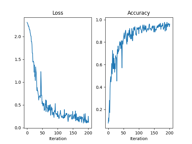
fig = plt.figure()
axes = [fig.add_subplot(1, 2, 1), fig.add_subplot(1, 2, 2)]

axes[0].plot(losses)
axes[0].set_title("Loss")
axes[0].set_xlabel("Iteration")

axes[1].plot(accuracies)
axes[1].set_title("Accuracy")
axes[1].set_xlabel("Iteration")

Iteration   0/200 Minibatch Loss 2.313  Accuracy 0.078
Iteration  50/200 Minibatch Loss 0.574  Accuracy 0.836
Iteration 100/200 Minibatch Loss 0.360  Accuracy 0.883
Iteration 150/200 Minibatch Loss 0.241  Accuracy 0.891
Iteration 200/200 Minibatch Loss 0.252  Accuracy 0.938

Text(0.5, 23.52222222222222, 'Iteration')