Matrix-free second-order optimization

This example walks you through a second-order optimizer that uses the conjugate gradient (CG) method and matrix-free multiplication with the block diagonal of different curvature matrices to solve for the Newton step.

The optimizer is tested on the classic MNIST example from PyTorch. In particular, we will use a model that suffers from the vanishing gradient problem and is hence difficult to optimizer for gradient descent. Second-order methods are less affected by that issue and can train these models, as they rescale the gradient according to the local curvature.

A local quadratic model of the loss defined by a curvature matrix \(C(x_t)\) (the Hessian, generalized Gauss-Newton, or other approximations)is minimized by taking the Newton step

\[x_{t+1} = x_t - \gamma (C(x_t) + \lambda I)^{-1} g(x_t),\]

where

\[\begin{split}\begin{array}{ll} x_t: & \text{parameters of the model} \\ g(x_t): & \text{gradient} \\ C(x_t): & \text{curvature of the local quadratic model at `x_t`} \\ \lambda: & \text{damping parameter} \\ \gamma: & \text{step-size} \\ \end{array}\end{split}\]

Let’s get the imports, configuration and some helper functions out of the way first. Notice that we are choosing a net with many sigmoids to make it hard to train for SGD.

Note

Larger batch sizes are usually recommended for second-order methods. However, the memory constraints imposed by the architecture used to build this example restrict us to rather small values.

import math

import matplotlib.pyplot as plt
import torch

from backpack import backpack, extend, extensions
from backpack.utils.examples import get_mnist_dataloder

BATCH_SIZE = 64
LR = 0.1
DAMPING = 1e-2
CG_TOL = 0.1
CG_ATOL = 1e-6
CG_MAX_ITER = 20
MAX_ITER = 50
PRINT_EVERY = 10
DEVICE = torch.device("cuda:0" if torch.cuda.is_available() else "cpu")

torch.manual_seed(0)

mnist_loader = get_mnist_dataloder(batch_size=BATCH_SIZE)


def make_model():
    return torch.nn.Sequential(
        torch.nn.Conv2d(1, 10, 5, 1),
        torch.nn.Sigmoid(),
        torch.nn.MaxPool2d(2, 2),
        torch.nn.Conv2d(10, 20, 5, 1),
        torch.nn.Sigmoid(),
        torch.nn.MaxPool2d(2, 2),
        torch.nn.Flatten(),
        torch.nn.Linear(4 * 4 * 20, 50),
        torch.nn.Sigmoid(),
        torch.nn.Linear(50, 10),
    )


model = make_model().to(DEVICE)

loss_function = torch.nn.CrossEntropyLoss().to(DEVICE)


def get_accuracy(output, targets):
    """Helper function to print the accuracy"""
    predictions = output.argmax(dim=1, keepdim=True).view_as(targets)
    return predictions.eq(targets).float().mean().item()

Writing the optimizer

To compute the update, we need access to the curvature matrix in form of matrix-vector products. We can then solve the linear system implied by the Newton step with CG,

\[(C(x_t) + \lambda I) v = - g(x_t),\]

and perform the update

\[x_{t+1} = x_t - \gamma v,\]

for every parameter.

Here is the optimizer. At its core is a simple implementation of CG that will iterate until the residual norm decreases a certain threshold (determined the atol and tol arguments), or exceeds a maximum budget (maxiter).

class CGNOptimizer(torch.optim.Optimizer):
    def __init__(
            self,
            parameters,
            bp_extension,
            lr=0.1,
            damping=1e-2,
            maxiter=100,
            tol=1e-1,
            atol=1e-8,
    ):
        super().__init__(
            parameters,
            dict(
                lr=lr,
                damping=damping,
                maxiter=maxiter,
                tol=tol,
                atol=atol,
                savefield=bp_extension.savefield,
            ),
        )
        self.bp_extension = bp_extension

    def step(self):
        for group in self.param_groups:
            for p in group["params"]:
                damped_curvature = self.damped_matvec(
                    p, group["damping"], group["savefield"]
                )

                direction, info = self.cg(
                    damped_curvature,
                    -p.grad.data,
                    maxiter=group["maxiter"],
                    tol=group["tol"],
                    atol=group["atol"],
                )

                p.data.add_(direction, alpha=group["lr"])

    def damped_matvec(self, param, damping, savefield):
        curvprod_fn = getattr(param, savefield)

        def matvec(v):
            v = v.unsqueeze(0)
            result = damping * v + curvprod_fn(v)
            return result.squeeze(0)

        return matvec

    @staticmethod
    def cg(A, b, x0=None, maxiter=None, tol=1e-5, atol=1e-8):
        r"""Solve :math:`Ax = b` for :math:`x` using conjugate gradient.

        The interface is similar to CG provided by :code:`scipy.sparse.linalg.cg`.

        The main iteration loop follows the pseudo code from Wikipedia:
            https://en.wikipedia.org/w/index.php?title=Conjugate_gradient_method&oldid=855450922

        Parameters
        ----------
        A : function
            Function implementing matrix-vector multiplication by `A`.
        b : torch.Tensor
            Right-hand side of the linear system.
        x0 : torch.Tensor
            Initialization estimate.
        atol: float
            Absolute tolerance to accept convergence. Stop if
            :math:`|| A x - b || <` `atol`
        tol: float
            Relative tolerance to accept convergence. Stop if
            :math:`|| A x - b || / || b || <` `tol`.
        maxiter: int
            Maximum number of iterations.

        Returns
        -------
        x (torch.Tensor): Approximate solution :math:`x` of the linear system
        info (int): Provides convergence information, if CG converges info
                    corresponds to numiter, otherwise info is set to zero.
        """
        maxiter = b.numel() if maxiter is None else min(maxiter, b.numel())
        x = torch.zeros_like(b) if x0 is None else x0

        # initialize parameters
        r = (b - A(x)).detach()
        p = r.clone()
        rs_old = (r ** 2).sum().item()

        # stopping criterion
        norm_bound = max([tol * torch.norm(b).item(), atol])

        def converged(rs, numiter):
            """Check whether CG stops (convergence or steps exceeded)."""
            norm_converged = norm_bound > math.sqrt(rs)
            info = numiter if norm_converged else 0
            iters_exceeded = numiter > maxiter
            return (norm_converged or iters_exceeded), info

        # iterate
        iterations = 0
        while True:
            Ap = A(p).detach()

            alpha = rs_old / (p * Ap).sum().item()
            x.add_(p, alpha=alpha)
            r.sub_(Ap, alpha=alpha)
            rs_new = (r ** 2).sum().item()
            iterations += 1

            stop, info = converged(rs_new, iterations)
            if stop:
                return x, info

            p.mul_(rs_new / rs_old)
            p.add_(r)
            rs_old = rs_new

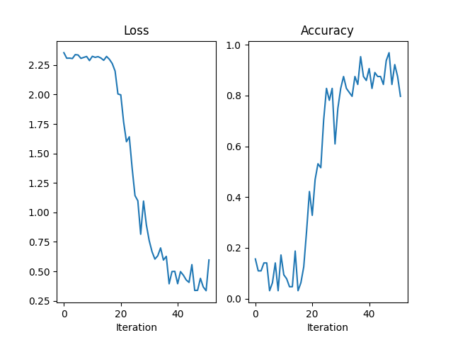
Running and plotting

Let’s try the Newton-style CG optimizer with the generalized Gauss-Newton (GGN) as curvature matrix.

After extend-ing the model and the loss function and creating the optimizer, we have to add the curvature-matrix product extension to the with backpack(...) context in a backward pass, such that the optimizer has access to the GGN product. The rest is just a canonical training loop which logs and visualizes training loss and accuracy.

model = extend(model)
loss_function = extend(loss_function)
optimizer = CGNOptimizer(
    model.parameters(),
    extensions.GGNMP(),
    lr=LR,
    damping=DAMPING,
    maxiter=CG_MAX_ITER,
    tol=CG_TOL,
    atol=CG_ATOL,
)

losses = []
accuracies = []
for batch_idx, (x, y) in enumerate(mnist_loader):
    optimizer.zero_grad()

    x, y = x.to(DEVICE), y.to(DEVICE)
    outputs = model(x)
    loss = loss_function(outputs, y)

    with backpack(optimizer.bp_extension):
        loss.backward()

    optimizer.step()

    # Logging
    losses.append(loss.detach().item())
    accuracies.append(get_accuracy(outputs, y))

    if (batch_idx % PRINT_EVERY) == 0:
        print(
            "Iteration %3.d/%3.d " % (batch_idx, MAX_ITER)
            + "Minibatch Loss %.5f  " % losses[-1]
            + "Accuracy %.5f" % accuracies[-1]
        )

    if MAX_ITER is not None and batch_idx > MAX_ITER:
        break

fig = plt.figure()
axes = [fig.add_subplot(1, 2, 1), fig.add_subplot(1, 2, 2)]

axes[0].plot(losses)
axes[0].set_title("Loss")
axes[0].set_xlabel("Iteration")

axes[1].plot(accuracies)
axes[1].set_title("Accuracy")
axes[1].set_xlabel("Iteration")

Out:

/home/docs/checkouts/readthedocs.org/user_builds/backpack/envs/1.2.0/lib/python3.7/site-packages/torch/nn/modules/module.py:795: UserWarning: Using a non-full backward hook when the forward contains multiple autograd Nodes is deprecated and will be removed in future versions. This hook will be missing some grad_input. Please use register_full_backward_hook to get the documented behavior.
  warnings.warn("Using a non-full backward hook when the forward contains multiple autograd Nodes "
Iteration   0/ 50 Minibatch Loss 2.35480  Accuracy 0.15625
Iteration  10/ 50 Minibatch Loss 2.32407  Accuracy 0.09375
Iteration  20/ 50 Minibatch Loss 1.99725  Accuracy 0.32812
Iteration  30/ 50 Minibatch Loss 0.75986  Accuracy 0.82812
Iteration  40/ 50 Minibatch Loss 0.39462  Accuracy 0.90625
Iteration  50/ 50 Minibatch Loss 0.33532  Accuracy 0.87500

Text(0.5, 23.52222222222222, 'Iteration')

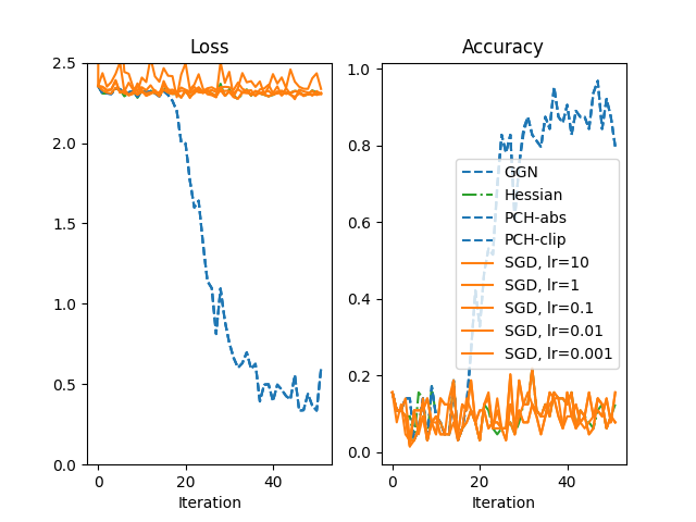
Vanishing gradients: comparison with SGD

By intention, we chose a model that is different to optimize with gradient descent due to the large number of sigmoids that reduce the gradient signal in backpropagation.

To verify that, let’s compare the Newton optimizer for different curvatures with SGD. SGD is run for a large range of learning rates lr ∈ [10, 1, 0.1, 0.01, 0.001].

The performance of CG-Newton versus SGD is shown below (using a somewhat simplified color scheme to simplify the visualization).

def make_cgn_optimizer_fn(extension):
    def optimizer_fn(model):
        return CGNOptimizer(
            model.parameters(),
            extension,
            lr=LR,
            damping=DAMPING,
            maxiter=CG_MAX_ITER,
            tol=CG_TOL,
            atol=CG_ATOL,
        )

    return optimizer_fn


curvatures = [
    extensions.GGNMP(),
    extensions.HMP(),
    extensions.PCHMP(modify="abs"),
    extensions.PCHMP(modify="clip"),
]

labels = [
    "GGN",
    "Hessian",
    "PCH-abs",
    "PCH-clip",
]

optimizers = []
for curvature in curvatures:
    optimizers.append(make_cgn_optimizer_fn(curvature))


def make_sgd_optimizer_fn(lr):
    def optimizer_fn(model):
        return torch.optim.SGD(model.parameters(), lr=lr)

    return optimizer_fn


sgd_lrs = [
    10,
    1,
    0.1,
    0.01,
    0.001,
]

for lr in sgd_lrs:
    optimizers.append(make_sgd_optimizer_fn(lr))
    labels.append("SGD, lr={}".format(lr))


def train(optim_fn):
    torch.manual_seed(0)

    mnist_loader = get_mnist_dataloder(batch_size=BATCH_SIZE)
    model = make_model().to(DEVICE)
    loss_function = torch.nn.CrossEntropyLoss().to(DEVICE)

    optimizer = optim_fn(model)
    need_backpack = isinstance(optimizer, CGNOptimizer)

    if need_backpack:
        model = extend(model)
        loss_function = extend(loss_function)

    losses = []
    accuracies = []
    for batch_idx, (x, y) in enumerate(mnist_loader):
        optimizer.zero_grad()

        x, y = x.to(DEVICE), y.to(DEVICE)
        outputs = model(x)
        loss = loss_function(outputs, y)

        if need_backpack:
            with backpack(optimizer.bp_extension):
                loss.backward()
        else:
            loss.backward()

        optimizer.step()

        # Logging
        losses.append(loss.detach().item())
        accuracies.append(get_accuracy(outputs, y))

        if (batch_idx % PRINT_EVERY) == 0:
            print(
                "Iteration %3.d/%3.d " % (batch_idx, MAX_ITER)
                + "Minibatch Loss %.5f  " % losses[-1]
                + "Accuracy %.5f" % accuracies[-1]
            )

        if MAX_ITER is not None and batch_idx > MAX_ITER:
            break

    return losses, accuracies


fig = plt.figure()
axes = [fig.add_subplot(1, 2, 1), fig.add_subplot(1, 2, 2)]

axes[0].set_title("Loss")
axes[0].set_ylim(0, 2.5)
axes[0].set_xlabel("Iteration")

axes[1].set_title("Accuracy")
axes[1].set_xlabel("Iteration")

for optim_fn, label in zip(optimizers, labels):
    print(label)
    losses, accuracies = train(optim_fn)

    if "SGD" in label:
        axes[0].plot(losses, "-", color="tab:orange", label=label)
        axes[1].plot(accuracies, "-", color="tab:orange", label=label)
    elif "Hessian" in label:
        axes[0].plot(losses, "-.", color="tab:green", label=label)
        axes[1].plot(accuracies, "-.", color="tab:green", label=label)
    else:
        axes[0].plot(losses, "--", color="tab:blue", label=label)
        axes[1].plot(accuracies, "--", color="tab:blue", label=label)

plt.legend()

Out:

GGN
/home/docs/checkouts/readthedocs.org/user_builds/backpack/envs/1.2.0/lib/python3.7/site-packages/torch/nn/modules/module.py:795: UserWarning: Using a non-full backward hook when the forward contains multiple autograd Nodes is deprecated and will be removed in future versions. This hook will be missing some grad_input. Please use register_full_backward_hook to get the documented behavior.
  warnings.warn("Using a non-full backward hook when the forward contains multiple autograd Nodes "
Iteration   0/ 50 Minibatch Loss 2.35480  Accuracy 0.15625
Iteration  10/ 50 Minibatch Loss 2.32407  Accuracy 0.09375
Iteration  20/ 50 Minibatch Loss 1.99725  Accuracy 0.32812
Iteration  30/ 50 Minibatch Loss 0.75986  Accuracy 0.82812
Iteration  40/ 50 Minibatch Loss 0.39462  Accuracy 0.90625
Iteration  50/ 50 Minibatch Loss 0.33532  Accuracy 0.87500
Hessian
Iteration   0/ 50 Minibatch Loss 2.35480  Accuracy 0.15625
Iteration  10/ 50 Minibatch Loss 2.32469  Accuracy 0.09375
Iteration  20/ 50 Minibatch Loss 2.32172  Accuracy 0.03125
Iteration  30/ 50 Minibatch Loss 2.33445  Accuracy 0.12500
Iteration  40/ 50 Minibatch Loss 2.29927  Accuracy 0.12500
Iteration  50/ 50 Minibatch Loss 2.31358  Accuracy 0.09375
PCH-abs
Iteration   0/ 50 Minibatch Loss 2.35480  Accuracy 0.15625
Iteration  10/ 50 Minibatch Loss 2.32406  Accuracy 0.09375
Iteration  20/ 50 Minibatch Loss 1.99709  Accuracy 0.32812
Iteration  30/ 50 Minibatch Loss 0.75543  Accuracy 0.84375
Iteration  40/ 50 Minibatch Loss 0.39352  Accuracy 0.90625
Iteration  50/ 50 Minibatch Loss 0.33675  Accuracy 0.87500
PCH-clip
Iteration   0/ 50 Minibatch Loss 2.35480  Accuracy 0.15625
Iteration  10/ 50 Minibatch Loss 2.32407  Accuracy 0.09375
Iteration  20/ 50 Minibatch Loss 1.99700  Accuracy 0.32812
Iteration  30/ 50 Minibatch Loss 0.75807  Accuracy 0.84375
Iteration  40/ 50 Minibatch Loss 0.39428  Accuracy 0.90625
Iteration  50/ 50 Minibatch Loss 0.33643  Accuracy 0.87500
SGD, lr=10
Iteration   0/ 50 Minibatch Loss 2.35480  Accuracy 0.15625
Iteration  10/ 50 Minibatch Loss 2.40687  Accuracy 0.07812
Iteration  20/ 50 Minibatch Loss 2.49646  Accuracy 0.03125
Iteration  30/ 50 Minibatch Loss 2.44262  Accuracy 0.12500
Iteration  40/ 50 Minibatch Loss 2.42848  Accuracy 0.09375
Iteration  50/ 50 Minibatch Loss 2.43353  Accuracy 0.09375
SGD, lr=1
Iteration   0/ 50 Minibatch Loss 2.35480  Accuracy 0.15625
Iteration  10/ 50 Minibatch Loss 2.34693  Accuracy 0.09375
Iteration  20/ 50 Minibatch Loss 2.32786  Accuracy 0.03125
Iteration  30/ 50 Minibatch Loss 2.31912  Accuracy 0.12500
Iteration  40/ 50 Minibatch Loss 2.30326  Accuracy 0.12500
Iteration  50/ 50 Minibatch Loss 2.29920  Accuracy 0.09375
SGD, lr=0.1
Iteration   0/ 50 Minibatch Loss 2.35480  Accuracy 0.15625
Iteration  10/ 50 Minibatch Loss 2.31614  Accuracy 0.09375
Iteration  20/ 50 Minibatch Loss 2.32291  Accuracy 0.03125
Iteration  30/ 50 Minibatch Loss 2.31921  Accuracy 0.12500
Iteration  40/ 50 Minibatch Loss 2.30273  Accuracy 0.12500
Iteration  50/ 50 Minibatch Loss 2.30004  Accuracy 0.09375
SGD, lr=0.01
Iteration   0/ 50 Minibatch Loss 2.35480  Accuracy 0.15625
Iteration  10/ 50 Minibatch Loss 2.32386  Accuracy 0.04688
Iteration  20/ 50 Minibatch Loss 2.32216  Accuracy 0.10938
Iteration  30/ 50 Minibatch Loss 2.32547  Accuracy 0.07812
Iteration  40/ 50 Minibatch Loss 2.29940  Accuracy 0.15625
Iteration  50/ 50 Minibatch Loss 2.30404  Accuracy 0.07812
SGD, lr=0.001
Iteration   0/ 50 Minibatch Loss 2.35480  Accuracy 0.15625
Iteration  10/ 50 Minibatch Loss 2.33067  Accuracy 0.04688
Iteration  20/ 50 Minibatch Loss 2.33119  Accuracy 0.10938
Iteration  30/ 50 Minibatch Loss 2.34716  Accuracy 0.07812
Iteration  40/ 50 Minibatch Loss 2.30991  Accuracy 0.15625
Iteration  50/ 50 Minibatch Loss 2.32288  Accuracy 0.07812

<matplotlib.legend.Legend object at 0x7fe8fb7d9c90>

While SGD is not capable to train this particular model, the second-order methods are still able to do so. Such methods may be interesting for optimization tasks that first-order methods struggle with.

Note that the Hessian of the net is not positive semi-definite. In this case, the local quadratic model does not have a global minimum and that complicates the usage of the Hessian in second-order optimization. This also provides a motivation for the other positive semi-definite Hessian approximations shown here.